Calibration – The Foundation of Quality Data

This column is devoted to helping cannabis analytical labs generate valid data right now with a relatively small amount of additional work. The topic for this article is instrument calibration – truly the foundation of all quality data. Calibration is the basis for all measurement, and it is absolutely necessary for quantitative cannabis analyses including potency, residual solvents, terpenes, and pesticides.
Just like a simple alarm clock, all analytical instruments – no matter how high-tech – will not function properly unless they are calibrated. When we set our alarm clock to 6AM, that alarm clock will sound reproducibly every 24 hours when it reads 6AM, but unless we set the correct current time on the clock based on some known reference, we can’t be sure when exactly the alarm will sound. Analytical instruments are the same. Unless we calibrate the instrument’s signal (the response) from the detector to a known amount of reference material, the instrument will not generate an accurate or valid result.
Without calibration, our result may be reproducible – just like in our alarm clock example – but the result will have no meaning unless the result is calibrated against a known reference. Every instrument that makes a quantitative measurement must be calibrated in order for that measurement to be valid. Luckily, the principle for calibration of chromatographic instruments is the same regardless of detector or technique (GC or LC).
Before we get into the details, I would like to introduce one key concept:
Every calibration curve for chromatographic analyses is expressed in terms of response and concentration. For every detector the relationship between analyte (e.g. a compound we’re analyzing) concentration and response is expressible mathematically – often a linear relationship.
Now that we’ve introduced the key concept behind calibration, let’s talk about the two most common and applicable calibration options.
Single Point Calibration
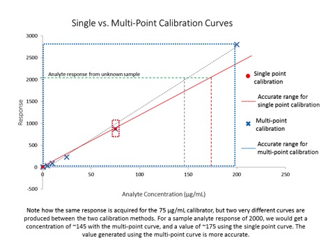
This is the simplest calibration option. Essentially, we run one known reference concentration (the calibrator) and calculate our sample concentrations based on this single point. Using this method, our curve is defined by two points: our single reference point, and zero. That gives us a nice, straight line defining the relationship between our instrument response and our analyte concentration all the way from zero to infinity. If only things were this easy. There are two fatal flaws of single point calibrations:
- We assume a linear detector response across all possible concentrations
- We assume at any concentration greater than zero, our response will be greater than zero
Assumption #1 is never true, and assumption #2 is rarely true. Generally, single point calibration curves are used to conduct pass/fail tests where there is a maximum limit for analytes (i.e. residual solvents or pesticide screening). Usually, quantitative values are not reported based on single point calibrations. Instead, reports are generated in relation to our calibrator, which is prepared at a known concentration relating to a regulatory limit, or the instrument’s LOD. Using this calibration method, we can accurately report that the sample contains less than or greater than the regulatory limit of an analyte, but we cannot report exactly how much of the analyte is present. So how can we extend the accuracy range of a calibration curve in order to report quantitative values? The answer to this question brings us to the other common type of calibration curve.
Multi-Point Calibration:
A multi-point calibration curve is the most common type used for quantitative analyses (e.g. analyses where we report a number). This type of curve contains several calibrators (at least 3) prepared over a range of concentrations. This gives us a calibration curve (sometimes a line) defined by several known references, which more accurately expresses the response/concentration relationship of our detector for that analyte. When preparing a multi-point calibration curve, we must be sure to bracket the expected concentration range of our analytes of interest, because once our sample response values move outside the calibration range, the results calculated from the curve are not generally considered quantitative.
The figure below illustrates both kinds of calibration curves, as well as their usable accuracy range:
This article provides an overview of the two most commonly used types of calibration curves, and discusses how they can be appropriately used to report data. There are two other important topics that were not covered in this article concerning calibration curves: 1) how can we tell whether or not our calibration curve is ‘good’ and 2) calibrations aren’t permanent – instruments must be periodically re-calibrated. In my next article, I’ll cover these two topics to round out our general discussion of calibration – the basis for all measurement. If you have any questions about this article or would like further details on the topic presented here, please feel free to contact me at amanda.rigdon@restek.com.