Tag Archives: calibration curve

The Practical Chemist

Building the Foundation of Medical Cannabis Testing – Understanding the Use of Standards and Reference Materials – Part 1

By Joe Konschnik
No Comments

In previous articles, you may recall that Amanda Rigdon, one our contributing authors, stated that instrument calibration is the foundation of all data quality. In this article, I would like to expand on that salient point. A properly calibrated instrument will, in fact, produce reliable data. It is the foundation we build our data upon. All foundations are comprised of building blocks, and our laboratory is no exception. If we take this analogy further, the keystone to the laboratory foundation, the stone that all data relies upon, is the analytical reference material. Proper calibration means that it is based on a true, accurate value. That is what the reference material provides. In this article, I would like to expand on the use and types of reference materials in analytical testing.

To develop sound analytical data, it is important to understand the significance of reference materials and how they are properly used. The proper selection and use of reference materials ensures the analytical certainty, traceability and comparability necessary to produce scientifically sound data. First, let’s take a moment to define the types of commonly used reference materials. According to the International Vocabulary of Metrology (VIM), a Reference Standard (RS) is something that is reused to measure against, like a balance or a set of weights. A Reference Material (RM) is a generic term. It is described as something that is prepared using a RS that is homogeneous, stable and is consumed during its use for measurement. An example of an RM is the solutions used to construct a calibration curve, often referred to as calibration standards, on your GC or LC. Due to the current state of cannabis testing, reference materials can be hard to find and, even more critical, variable in their accuracy to a known reference standard. Sometimes this is not critical, but when quantifying an unknown, it is paramount.

RMs can be either quantitative or qualitative. Qualitative RMs verify the identity and purity of a compound. Quantitative RMs, on the other hand, provide a known concentration, or mass, telling us not only what is present, and its purity, but also how much. This is typically documented on the certificate that accompanies the reference material, which is provided by the producer or manufacturer. The certificate describes all of the properties of the starting materials and steps taken to prepare the RM. For testing requirements, like potency, pesticides, etc., where quantitation is expected, it is important to use properly certified quantitative RMs.

Now, the pinnacle of reference materials is the Certified Reference Material (CRM). VIM defines a Certified Reference Material (CRM) as an RM accompanied by documentation issued by an authoritative body and provides one or more specified property values, with associated uncertainties and traceability using valid procedures. A CRM is generally recognized as providing the highest level of traceability and accuracy to a measurement – the strongest keystone you can get for your foundation. It is also important to recognize that the existence of a certificate does not make a reference material a CRM. It is the process used in manufacturing that makes it a CRM, and these are typically accreditations earned by specific manufacturers who have invested on this level of detail.

Now that we understand the types of reference materials we can choose, in the next article of this series we will describe what a CRM provider must do to ensure the material and how we can use them to develop reliable data. Without properly formulated and prepared CRMs, instrument calibration and the use of internal standards are less effective at ensuring the quality of your data.


If you have any questions please contact me, Joe Konschnik at (800) 356-1688 ext. 2002 by phone, or email me at joe.konschnik@restek.com.

amandarigdon
The Practical Chemist

Calibration Part II – Evaluating Your Curves

By Amanda Rigdon
No Comments
amandarigdon

Despite the title, this article is not about weight loss – it is about generating valid analytical data for quantitative analyses. In the last installment of The Practical Chemist, I introduced instrument calibration and covered a few ways we can calibrate our instruments. Just because we have run several standards across a range of concentrations and plotted a curve using the resulting data, it does not mean our curve accurately represents our instrument’s response across that concentration range. In order to be able to claim that our calibration curve accurately represents our instrument response, we have to take a look at a couple of quality indicators for our curve data:

  1. correlation coefficient (r) or coefficient of determination (r2)
  2. back-calculated accuracy (reported as % error)

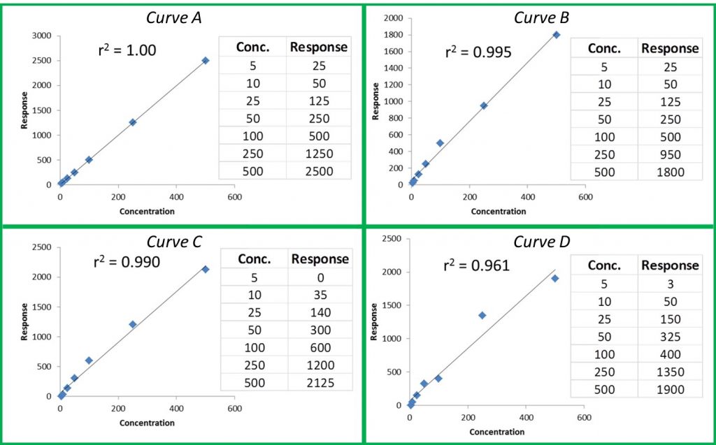
The r or r2 values that accompany our calibration curve are measurements of how closely our curve matches the data we have generated. The closer the values are to 1.00, the more accurately our curve represents our detector response. Generally, r values ≥0.995 and r2 values ≥ 0.990 are considered ‘good’. Figure 1 shows a few representative curves, their associated data, and r2 values (concentration and response units are arbitrary).

Figure 1: Representative Curves and r2 values

Let’s take a closer look at these curves:

Curve A: This represents a case where the curve perfectly matches the instrument data, meaning our calculated unknown values will be accurate across the entire calibration range.

Curve B: The r2 value is good and visually the curve matches most of the data points pretty well. However, if we look at our two highest calibration points, we can see that they do not match the trend for the rest of the data; the response values should be closer to 1250 and 2500. The fact that they are much lower than they should be could indicate that we are starting to overload our detector at higher calibration levels; we are putting more mass of analyte into the detector than it can reliably detect. This is a common problem when dealing with concentrated samples, so it can occur especially for potency analyses.

Curve C: We can see that although our r2 value is still okay, we are not detecting analytes as we should at the low end of our curve. In fact, at our lowest calibration level, the instrument is not detecting anything at all (0 response at the lowest point). This is a common problem with residual solvent and pesticide analyses where detection levels for some compounds like benzene are very low.

Curve D: It is a perfect example of our curve not representing our instrument response at all. A curve like this indicates a possible problem with the instrument or sample preparation.

So even if our curve looks good, we could be generating inaccurate results for some samples. This brings us to another measure of curve fitness: back-calculated accuracy (expressed as % error). This is an easy way to determine how accurate your results will be without performing a single additional run.

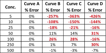
Back-calculated accuracy simply plugs the area values we obtained from our calibrators back into the calibration curve to see how well our curve will calculate these values in relation to the known value. We can do this by reprocessing our calibrators as unknowns or by hand. As an example, let’s back-calculate the concentration of our 500 level calibrator from Curve B. The formula for that curve is: y = 3.543x + 52.805. If we plug 1800 in for y and solve for x, we end up with a calculated concentration of 493. To calculate the error of our calculated value versus the true value, we can use the equation: % Error = [(calculated value – true value)/true value] * 100. This gives us a % error of -1.4%. Acceptable % error values are usually ±15 – 20% depending on analysis type. Let’s see what the % error values are for the curves shown in Figure 1.

practical chemist table 1
Table 1: % Error for Back-Calculated Values for Curves A – D

Our % error values have told us what our r2 values could not. We knew Curve D was unacceptable, but now we can see that Curves B and C will yield inaccurate results for all but the highest levels of analyte – even though the results were skewed at opposite ends of the curves.

There are many more details regarding generating calibration curves and measuring their quality that I did not have room to mention here. Hopefully, these two articles have given you some tools to use in your lab to quickly and easily improve the quality of your data. If you would like to learn more about this topic or have any questions, please don’t hesitate to contact me at amanda.rigdon@restek.com.